Fixed Effects Continuous Treatment Individual Level Panel
Regression Estimators
Fixed effects regressions generally start with a regression equation that looks like this:
\[\begin{equation} \tag{16.1} Y_{it} = \beta_i + \beta_1X_{it} + \varepsilon_{it} \end{equation}\]
This looks exactly like our standard regression equation from Chapter 13 with two main exceptions. The first is that \(X\) has the subscript \(it\), indicating that the data varies both between individuals (\(i\)) and over time (\(t\)).
The second is that the intercept term \(\beta\) now has a subscript \(i\) instead of an 0, making it \(\beta_i\). Thinking of regression as a way of fitting a straight line, this means that all the individuals in the data are constrained to have the same slope (there's no \(i\) subscript on \(\beta_1\)), but they have different intercepts.
Three obvious questions arise.
QUESTION 1. How does allowing the intercept to vary give you a fixed effects estimate where you use only within variation?
There are two ways to think about this intuitively. The first is procedural. By allowing the intercept to vary it's sort of like we're adding a control for each person. Let's take a study of countries for example. If India is in our sample, then one of the intercepts is \(\beta_{India}\). This intercept only applies to India, not to any of the other countries.
That's a lot like adding a "This is India" binary control variable to our regression, and \(\beta_{India}\) is the coefficient on that control variable. We have one of these controls for each country in our data. So we're controlling for each different country. And we know what happens when we control for country. We get within-country variation.
The second way to think about why this works intuitively is to think in terms of a graph. Figure 16.8 uses data on GDP per capita and life expectancy from the Gapminder Institute (Gapminder Institute 2020Gapminder Institute. 2020. "Gapminder." https://www.gapminder.org/.). Here we've isolated just two countries - India and Brazil, and are looking at their data since 1952.
Figure 16.8: GDP per Capita and Life Expectancy in Two Countries
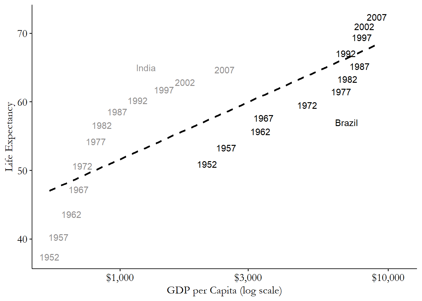
We can see a few things clearly in Figure 16.8. First, things in both countries are clearly getting better over time. 443 Neat! However, there are also some clear between-country differences we want to get rid of. And that regression line, with a single intercept for both, is clearly underestimating the slope of the lines that each of the two of them have.
By breaking up the intercept, we can instead use two lines - parallel lines, since they have the same slope - and move them up and down until we hit each country. This lets us not care how far up or down each country's cluster of points is since we can just move up and down to hit it (we get within variation in the \(y\)-axis variable), and also lets us not care how far left or right each country's cluster is, since by moving up and down, the same slope can hit the cluster no matter how far out to the right it is (we get within variation in the \(x\)-axis variable). And thus we have within variation.
Figure 16.9: GDP per Capita and Life Expectancy in Two Countries
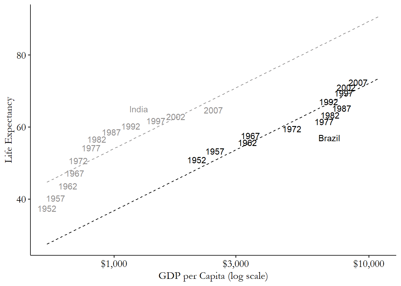
We do exactly this - the same slope but with different intercepts - in Figure 16.9. The lines are a lot closer to those points now. Those lines capture the relationship that's clearly there a lot better than the single regression line did.
QUESTION 2. How do we estimate a regression with individual intercepts?
There are actually a bunch of ways to do this. Some of them we will cover in later parts of this chapter. 444 Some of them don't even isolate only the within-variation. Scandalous! But within that long list of ways, there are two standard methods, both of which are dead-simple and only use tools we already know.
The first method is just to extract the within variation ourselves, and work with that. 445 This approach gets way trickier if you have more than one set of fixed effects. Just calculate the mean of the dependent variable for each individual (\(\bar{Y}_i\)) and subtract that mean out (\(Y_{it}-\bar{Y}_i\)). Then do the same for each of the independent variables (\(X_{it}-\bar{X}_i\)). Then run the regression
\[\begin{equation} \tag{16.2} Y_{it}-\bar{Y}_i = \beta_0 + \beta_1(X_{it}-\bar{X}_i) + \varepsilon_{it} \end{equation}\]
This method is known as "absorbing the fixed effect." 446 \(\beta_0\) is sometimes left out of the equation when doing this method, because it will be 0 anyway. Think about why that should be. Let's run this approach using the Gapminder data once again.
R Code
library(tidyverse); library(modelsummary) gm <- causaldata::gapminder gm <- gm %>% # Put GDP per capita in log format since it's very skewed mutate(log_GDPperCap = log(gdpPercap)) %>% # Perform each calculation by group group_by(country) %>% # Get within variation by subtracting out the mean mutate(lifeExp_within = lifeExp - mean(lifeExp), log_GDPperCap_within = log_GDPperCap - mean(log_GDPperCap)) %>% # We no longer need the grouping ungroup() # Analyze the within variation m1 <- lm(lifeExp_within ~ log_GDPperCap_within, data = gm) msummary(m1, stars = c('*' = .1, '**' = .05, '***' = .01)) Stata Code
causaldata gapminder.dta, use clear download * Get log GDP per capita since GDP per capita is very skewed g logGDPpercap = log(gdppercap) * Get mean life expectancy and log GDP per capita by country by country, sort: egen lifeexp_mean = mean(lifeexp) by country, sort: egen logGDPpercap_mean = mean(logGDPpercap) * Subtract out that mean to get within variation g lifeexp_within = lifeexp - lifeexp_mean g logGDPpercap_within = logGDPpercap - logGDPpercap_mean * Analyze the within variation regress lifeexp_within logGDPpercap_within Python Code
import numpy as np import statsmodels.formula.api as sm from causaldata import gapminder gm = gapminder.load_pandas().data # Put GDP per capita in log format since it's very skewed gm['logGDPpercap'] = gm['gdpPercap'].apply('log') # Use groupby to perform calculations by group # Then use transform to subtract each variable's # within-group mean to get within variation gm[['logGDPpercap_within','lifeExp_within']] = (gm. groupby('country')[['logGDPpercap','lifeExp']]. transform(lambda x: x - np.mean(x))) # Analyze the within variation m1 = sm.ols(formula = 'lifeExp_within ~ logGDPpercap_within', data = gm).fit() m1.summary() The second simple method is to add a binary control variable for every country (individual). Or rather, every country except one - if our model also has an intercept/constant in it, then including every country will make the model impossible to estimate, so we leave one out, or leave the intercept out. 447 Why? Imagine we just have two people - me and you - and are estimating height. Say my average height over time is 66 inches and yours is 68, and we don't leave anyone out so we have \(Height_{it} = \beta_0 + \beta_1Me_i + \beta_2You_i\). The values \(\beta_0 = 0, \beta_1 = 66, \beta_2 = 68\) gives exactly the same fit as \(\beta_0 = 1, \beta_1 = 65, \beta_2 = 67\). There are infinite ways to get the exact same fit. There's no way it can choose! So the model can't be estimated. That one left-out country is still in the analysis, it just doesn't get its own coefficient. It's stuck with the lousy constant. Thankfully, most software will do this automatically.
I should point out that this is rarely the way you want to go. Including a set of binary indicators in the model is fine when you have a few different categories, but if you're controlling for each individual you may have hundreds or thousands of terms. This can get very, very slow. And c'mon, were you really going to interpret all those coefficients anyway? But for demonstrative purposes, we'll run this version to see what we get.
R Code
library(tidyverse); library(modelsummary) gm <- causaldata::gapminder # Simply include a factor variable in the model to get it turned # to binary variables. You can use factor() to ensure it's done. m2 <- lm(lifeExp ~ factor(country) + log(gdpPercap), data = gm) msummary(m2, stars = c('*' = .1, '**' = .05, '***' = .01)) Stata Code
causaldata gapminder.dta, use clear download g logGDPpercap = log(gdppercap) * Stata requires variables to be numbers before automatically * automatically making binary variables. So we encode. encode country, g(country_number) regress lifeexp logGDPpercap i.country_number Python Code
import numpy as np import statsmodels.formula.api as sm from causaldata import gapminder gm = gapminder.load_pandas().data gm['logGDPpercap'] = gm['gdpPercap'].apply('log') # Use C() to include binary variables for a categorical variable m2 = sm.ols(formula = "'lifeExp ~ logGDPpercap + C(country)"', data = gm).fit() m2.summary() Let's take a look at our results from the two methods, using the R output, in Table 16.3. With our second method we also estimated a bunch of country coefficients, but those aren't on the table (there are a lot of them).
| Life Expectancy (within) | Life Expectancy | |
|---|---|---|
| Log GDP per Capita (within) | 9.769*** | |
| (0.284) | ||
| Log GDP per Capita | 9.769*** | |
| (0.297) | ||
| Num.Obs. | 1704 | 1704 |
| R2 | 0.410 | 0.846 |
| RMSE | 5.06 | 5.29 |
| * p < 0.1, ** p < 0.05, *** p < 0.01 |
There are some minor differences between the two in terms of their standard errors, and some big differences in \(R^2\), but the coefficients are the same. 448 These code snippets are designed to be illustrative to show how both methods are equivalent. Most of the time, researchers will actually use one of the commands shown in the "Multiple Sets of Fixed Effects" section below, even if they only have one set of fixed effects. So now that we have the coefficients, how can we interpret them?
QUESTION 3. How do we interpret the results of this regression once we have estimated it?
The interpretation of the slope coefficient in a fixed effects model is the same as when you control for any other variable - within the same value of country, how is variation in log GDP per capita related to variation in life expectancy?
Put another way, since we have a coefficient of 9.769, we can say that for a given country, in a year where log GDP per capita is one unit higher than it typically is for that country, then we'd expect life expectancy to be 9.769 years longer than it typically is for that country. 449 As you'll recall from Chapter 13, a one-unit increase in log GDP per capita is a percentage increase in GDP per capita. Specifically, a 171% increase. But for smaller increases, the value and percentage are very close, so we might more often say a log GDP per capita .1 above the typical level, or GDP per capita roughly 10% above, is associated with an life expectancy of .9769 years above the typical level.
What else do we have on the table?
We can see that the \(R^2\) values are quite different in the two columns. Why is this?
Remember that \(R^2\) is a measure based on how much variation there is in our residuals relative to our dependent variable. 450 \(R^2 = 1 -\) var(residuals) / var(dependent variable), where var is short for variance. In the first column, our dependent variable is \(lifeExp_within\), not \(lifeExp\). So the \(R^2\) is based on how much variation there is in the residuals relative to the the within variation, not the overall variation in \(lifeExp\). This is called the "within \(R^2\)." On the contrary, the second column tells us how much variation there is in (those very same) residuals relative to all the variation in \(lifeExp\). It counts the parts of \(lifeExp\) explained by between variation (our binary variables).
Lastly, let's think about something that's not on the table - the fixed effects themselves. That is, those coefficients on the country binary variables we got in the second regression. For example, India's is 13.971 and Brazil's is 6.318. These are the intercepts in the country-specific fitted lines, like in Figure 16.9.
What can we make of these fixed effects? Not too much in absolute terms, 451 We can't consider them independently because they're all defined relative to whichever country didn't get its own coefficient - remember that? So Brazil's 6.318 doesn't mean its intercept is 6.318, it means its intercept is 6.318 higher than the intercept of the country that was left out. but they make sense relative to each other. So India's intercept is \(13.971 - 6.318 = 7.653\) higher than Brazil's.
We can interpret that to mean that, if India and Brazil had the same GDP per capita, we'd predict that India's life expectancy would be 7.653 higher than Brazil's. We're still looking at the effect of one variable controlling for another - just now, we're looking at the effect of country controlling for GDP per capita rather than the other way around.
Sometimes researchers will use these fixed effects estimates to make claims about the individuals being evaluated. They might say, for example, that India has especially high life expectancy given its level of GDP per capita.
This can be an interesting way to look at differences between individuals. However, keep in mind that fixed effects is a good way of controlling for a long list of unobserved variables that are fixed over time to look at the effect of a few time-varying variables. Those individual effects don't have the same luxury of controlling for a bunch of unobserved time-varying variables. We can rarely think of these individual fixed effects estimates as causal. 452 In addition, individual fixed effects estimates are estimated based on a relatively small number of observations - just the number we have per individual. So they tend to be a little wild and vary too much. Random effects - discussed later in the chapter - addresses this problem by "shrinkage" of the individual effects.
One last thing to keep in mind about fixed effects. It focuses on within variation. So the treatment effect (Chapter 10) estimated will focus a lot more heavily on people with a lot of within variation. In that life expectancy and GDP example, the coefficient on GDP we got is closer to estimating the effect of GDP on life expectancy in countries where GDP changed a lot over time. If your GDP was fairly constant, you count less for the estimate! You can address this by using weights to address the problem. 453 The Gibbons, Suárez, and Urbancic (2019Gibbons, Charles E., Serrato Juan Carlos Suárez, and Michael B. Urbancic. 2019. "Broken or Fixed Effects?" Journal of Econometric Methods 8 (1): 1–12.) paper suggests two solutions, the simplest of which is to calculate the variance of the treatment variable within individual, and weight by the inverse of that. This is an inverse variance weight, like in Chapter 13.
Multiple Sets of Fixed Effects
We've discussed fixed effects as being a way of controlling for a categorical variable. This ends up giving us the variation that occurs within that variable. So if we have fixed effects for individual, we are comparing that individual to themselves over time. And if we have fixed effects for city, we are comparing individuals in that city only to other individuals in that city.
So why not include multiple sets of fixed effects? Say we observe the same individuals over multiple years. We could include fixed effects for individual - comparing individuals to themselves at different periods of time, or fixed effects for year - comparing individuals to each other at the same period of time. What if we include fixed effects for both individual and year?
This approach - including fixed effects for both individual and for time period - is a common application of multiple sets of fixed effects, and is commonly known as two-way fixed effects. The regression model for two-way fixed effects looks like:
\[\begin{equation} \tag{16.3} Y_{it} = \beta_i + \beta_t + \beta_1X_{it} + \varepsilon_{it} \end{equation}\]
What does this get us? Well, we are looking at variation within individual as well as within year at this point. So we can think of the variation that's left as being variation relative to what we'd expect given that individual, and given that year. 454 Crucially, this is not the same as given that individual that year, as we only observe that individual in that year once. There's no variation. Each of the "relative to"s is one at a time.
For example, let's say we have data on how much each person earns per year (\(Y_{it}\)), and we also have data on how many hours of training they received that year (\(X_{it}\)). We want to know the effect of experience of in-job training on pay at that job.
We do happen to know that the year 2009 was a particularly bad year for earnings, what with the Great Recession and all. Let's say that earnings in 2009 were $10,000 below what they normally are. And let's say that we're looking at Anthony, who happens to earn $120,000 per year, a lot more money than the average person ($40,000).
In 2009 Anthony only earned $116,000. That's way above average, but that can be explained by the fact that it's Anthony and Anthony earns a lot. So given that it's Anthony, it's $4,000 below average. But given that it's 2009, most people are earning $10,000 less, but Anthony is only earning $4,000 less. So given that it's Anthony, and given that it's 2009, Anthony in 2009 is $6,000 more than you'd expect.
Or at least that's a rough explanation. Two-way fixed effects actually gets a fair amount more complex than that, since the individual fixed effects affect the year fixed effects and vice versa. Just like with one set of fixed effects, the variation that actually ends up getting used to estimate the treatment effect (Chapter 10) focuses more heavily on individuals that have a lot of variation over time. So if Anthony's level of in-job training is pretty steady over time, but some other person, Kamala, has a level of training that changes a lot from year to year, then the two-way fixed effects estimate will represent Kamala's treatment effect a lot more than Anthony's (De Chaisemartin and d'Haultfoeuille 2020De Chaisemartin, Clément, and Xavier d'Haultfoeuille. 2020. "Two-Way Fixed Effects Estimators with Heterogeneous Treatment Effects." American Economic Review 110 (9): 2964–96.).
Two-way fixed effects, with individual and time as the fixed effects, aren't the only way to have multiple sets of fixed effects, of course. As described above, for example, you could have fixed effects for individual and also for city. Neither of those is time!
The interpretation here is a lot closer to thinking of just including controls for individual and controls for city.
One thing to remember, though. We're isolating variation within individual and also within city. So in order for you to have any variation at all to be included, you need to show up in multiple cities. This is a more common problem here (two sets of fixed effects, neither of them is time) than with two-way fixed effects (individual and time), since generally each person shows up in each time period only once anyway.
If we ran our income-and-job-training study with individual and city fixed effects, the treatment effect would only be based on people who are observed in different cities at different times. Never move? You don't count!
Estimating a model with multiple fixed effects can be done using the same "binary controls" approach as for the regular ("one-way") fixed effects estimator with only one set of fixed effects. No problem!
However, this can be difficult if there are lots of different fixed effects to estimate. The computational problem gets thorny real fast. Unless your fixed effects only have a few categories each (say, fixed effects for left- or right-handedness and for eye color), it's generally advised that you use a command specifically designed to handle multiple sets of fixed effects.
These methods usually use something called alternating projections, which is sort of like our original method of calculating within variation and using that, except that it manages to take into account the way that the first set of fixed effects gives you within-variation in the other set, and vice versa.
Let's code this up, continuing with our Gapminder data.
R Code
library(tidyverse); library(modelsummary); library(fixest) gm <- causaldata::gapminder # Run our two-way fixed effects model (TWFE). # First the non-fixed effects part of the model # Then a |, then the fixed effects we want twfe <- feols(lifeExp ~ log(gdpPercap) | country + year, data = gm) # Note that standard errors will be clustered by the first # fixed effect by default. Set se = 'standard' to not do this msummary(twfe, stars = c('*' = .1, '**' = .05, '***' = .01)) Stata Code
causaldata gapminder.dta, use clear download g logGDPpercap = log(gdppercap) * We will use reghdfe which must be installed with * ssc install reghdfe reghdfe lifeexp logGDPpercap, a(country year) Python Code
import linearmodels as lm from causaldata import gapminder gm = gapminder.load_pandas().data gm['logGDPpercap'] = gm['gdpPercap'].apply('log') # Set our individual and time (index) for our data gm = gm.set_index(['country','year']) # Specify the regression model # And estimate with both sets of fixed effects # EntityEffects and TimeEffects # (this function can't handle more than two) mod = lm.PanelOLS.from_formula( "'lifeExp ~ logGDPpercap + EntityEffects + TimeEffects"',gm) twfe = mod.fit() print(twfe) Random Effects
As a research design, fixed effects is all about isolating within variation. We think that there are some back doors floating around in that between variation, so we get rid of it and focus on the within variation. But as a statistical method, fixed effects can really be thought of as a model in which the intercept varies freely across individuals. As I've put it before, here's the model:
\[\begin{equation} \tag{16.4} Y_{it} = \beta_i + \beta_1X_{it} + \varepsilon_{it} \end{equation}\]
It turns out that fixed effects is, statistically, a relatively weak way of letting that intercept vary. After all, we're only allowing within variation. And how many observations per individual do we really have? We may be estimating those \(\beta_i\)s with only a few observations, making them noisy, which in turn could make our estimate of \(\beta_1\) noisy too.
Random effects takes a slightly different approach. Instead of letting the \(\beta_i\)s be anything, it puts some structure on them. Specifically, it assumes that the \(\beta_i\)s come from a known random distribution, for example assuming that the \(\beta_i\)s follow a normal distribution.
This does a few things:
- It makes estimates more precise (lowers the standard errors).
- It improves the estimation of the individual \(\beta_i\) effects themselves. 455 Why? Because we assume that they come from the same distribution. We can use all the data to estimate that distribution, which means each estimate of \(\beta_i\) gets a lot more information to work off of.
- Instead of just using within variation, it uses a weighted average of within and between variation.
- It solves the same back door problem that fixed effects does if the \(\beta_i\) terms are unrelated to the right-hand-side variables \(X_{it}\).
That last item is a bit of a doozy. Sure, better statistical precision is nice. But we're only doing fixed effects in the first place to solve our research design problem. Random effects only solves the same problem if the individual fixed effects are unrelated to our right-hand-side variable, including our treatment variable.
That seems unlikely. Consider our Gapminder example. For random effects to be appropriate, the "country effect" would need to be unrelated to GDP. That is, all the stuff about a country that's fixed over time and determines its life expectancy other than GDP per capita needs to be completely unrelated to GDP per capita. And that list would include things like industrial development and geography. Those seem likely to be related to GDP per capita.
For this reason, fixed effects is almost always preferred to random effects, 456 Or at least this version of random effects… keep reading. except when you can be pretty sure that the right-hand-side variables are unrelated to the individual effect. For example, when you've run a randomized experiment, \(X_{it}\) is a truly randomly-assigned experimental variable and so is unrelated to any individual effect.
One common way around this problem is the use of the Durbin-Wu-Hausman test. The Durbin-Wu-Hausman test is a broad set of tests that compare the estimates in one model against the estimates in another and sees if they are different. In the context of fixed effects and random effects, if the estimates are found to not be different (you fail to reject the null hypothesis that they're the same), then the relationship between \(\beta_i\) and \(X_{it}\) probably isn't too strong, so you can go ahead and use random effects with its nice statistical properties.
However, I do not recommend the use of the Durbin-Wu-Hausman test for this purpose. 457 I do not like this testing plan, I do not like it Jerr Hausman. For one thing, if we don't have a strong theoretical reason to believe that the unrelated-\(\beta_i\)-and-\(X_{it}\) assumption holds, it's hard to really believe that failing to reject a null hypothesis can justify it for you.
For another, the Durbin-Wu-Hausman test compares fixed effects to the simplest version of random effects, which doesn't really use random effects to its full advantage. Most studies that use random effects use them in more useful ways that get around that doozy of an assumption. For that, you'll want to look at "Advanced Random Effects" in the "How the Pros Do It" section.
Source: https://theeffectbook.net/ch-FixedEffects.html
0 Response to "Fixed Effects Continuous Treatment Individual Level Panel"
Post a Comment